Exoplanets rarely pose for telescopes. Most are too small, too distant, and thoroughly overwhelmed by the glare of their host stars. Trying to see an Earth-sized planet beside a Sun-like star is a little like searching for a firefly hovering next to a stadium spotlightexcept the stadium is light-years away and refuses to turn down the brightness.
Astronomers therefore discover most extrasolar planets indirectly. They measure a star’s brightness, motion, position, or gravitational effect and ask whether the numbers behave as they would if an unseen planet were present. The essential tools include geometry, orbital mechanics, probability, statistics, and signal processing. Together, they turn tiny variations in starlight into estimates of a planet’s radius, mass, orbit, density, and temperature.
Why Exoplanet Hunting Is a Mathematical Problem
A telescope records photons, not labeled planets. Its raw output may contain a time, a wavelength, a pixel position, and a measured intensity. The planet emerges only after researchers construct a mathematical model and compare it with those observations.
Suppose a star dims every 10 days. That repetition may indicate a transiting planet, but it could also come from starspots, an eclipsing binary, an instrument problem, or another star contaminating the image. A credible discovery requires more than spotting an interesting wiggle. Astronomers must demonstrate that the signal is periodic, physically plausible, statistically significant, and more convincing than competing explanations.
The guiding idea is simple: an invisible object can still reveal itself through measurable consequences. The implementation involves considerably more algebraand occasionally enough coffee to qualify as a minor observatory expense.
Kepler’s Laws: The Foundation of Exoplanet Math
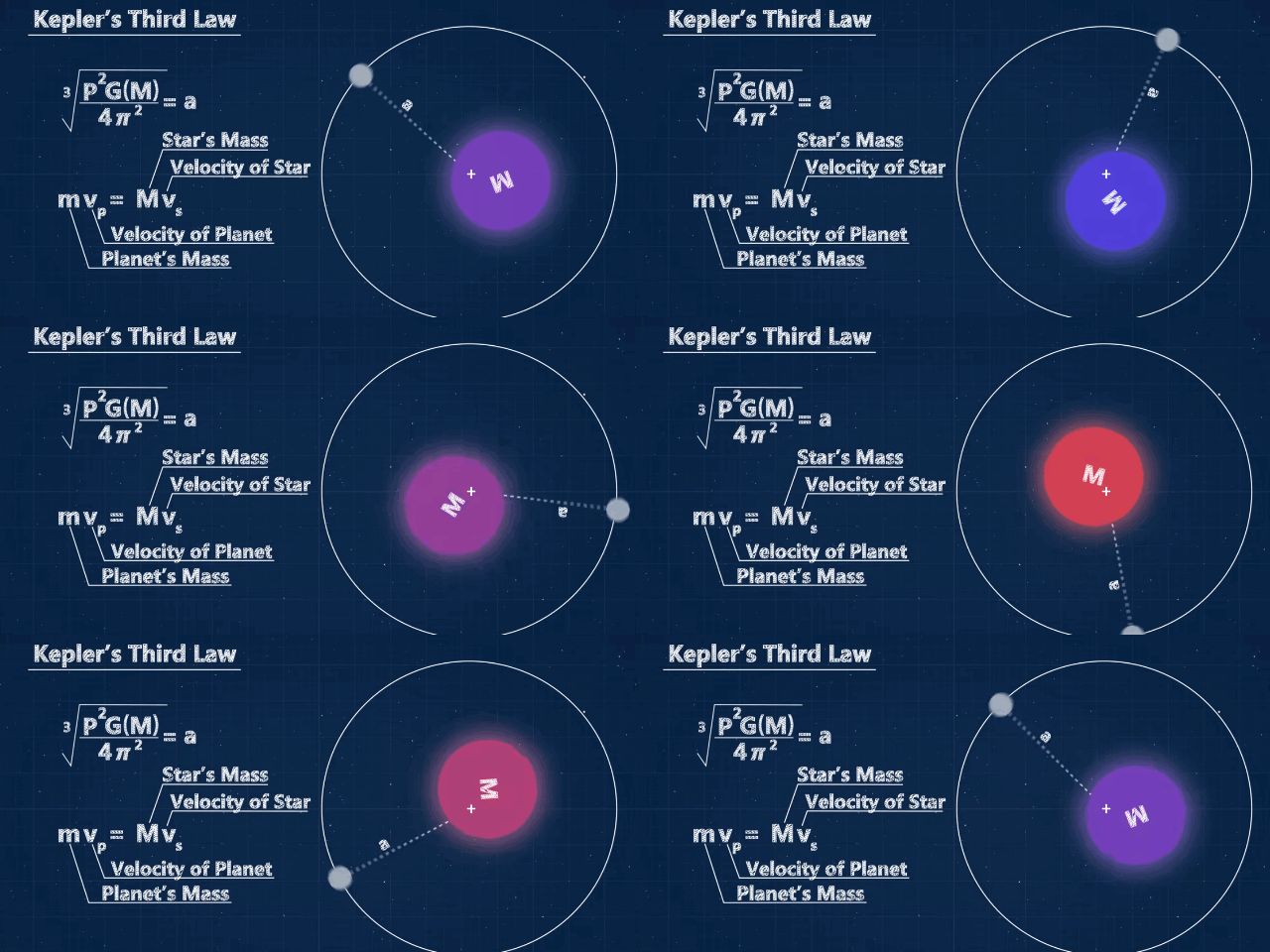
Planet hunters rely heavily on the orbital relationships described by Johannes Kepler and later explained through Newtonian gravity. The generalized form of Kepler’s third law is:
P2 = 4π2a3 / G(M* + Mp)
Here, P is the orbital period, a is the orbit’s semimajor axis, G is the gravitational constant, M* is the stellar mass, and Mp is the planet’s mass. Because a planet is usually much less massive than its star, astronomers often approximate the denominator using only M*.
This relationship is extremely useful. If repeated observations reveal the orbital period and stellar models provide the star’s mass, researchers can calculate the planet’s average orbital distance. A short period generally means a tight orbit; a long period points to a wider one.
The Barycenter and the Wobbling Star
A planet does not orbit the exact center of a motionless star. Both bodies orbit their shared center of mass, called the barycenter. Their distances from that point satisfy:
M*a* = Mpap
A massive planet pulls the barycenter farther from the star’s center, producing a larger stellar wobble. That motion powers two major detection techniques: radial velocity, which measures movement toward and away from Earth, and astrometry, which measures sideways movement across the sky.
Transit Photometry: Measuring a Planetary Shadow
The transit method looks for a small decrease in starlight when a planet crosses the face of its host star. The resulting graph of brightness over time is called a light curve. If the planet and star are approximated as disks with uniform brightness, the fractional transit depth is:
δ ≈ (Rp / R*)2
In this equation, δ is the fraction of light blocked, Rp is the planet’s radius, and R* is the star’s radius. Rearranging the formula gives:
Rp ≈ R*√δ
A Jupiter-sized planet passing in front of a Sun-sized star blocks roughly 1 percent of the star’s light. Earth crossing the Sun would produce a dip of only about 0.0084 percent, or 84 parts per million. Detecting that change is equivalent to noticing that someone quietly removed a few bulbs from an enormous illuminated sign.
Period, Distance, and Transit Duration
The time between successive dips provides the orbital period. Once P is known, Kepler’s third law estimates a. Transit duration adds more information. For a circular orbit crossing near the center of the star, a useful approximation is:
T ≈ (P / π)(R* / a)
Real calculations include the planet’s size, orbital inclination, eccentricity, and impact parameterthe projected distance between the planet’s path and the center of the stellar disk. Astronomers also model limb darkening, the fact that a star looks brighter in the center than near its edge. Consequently, a real transit is curved rather than a perfectly rectangular dip.
The Geometry Problem
Most planets never transit from Earth’s perspective because their orbital planes are not aligned with our line of sight. For a roughly circular orbit, the transit probability is approximately:
ptransit ≈ (R* + Rp) / a
Close-in planets are therefore much more likely to transit than distant ones. This geometric bias helps explain why transit surveys commonly find hot planets on short orbits. It does not mean the universe has a peculiar obsession with planets that could melt cookware.
Radial Velocity: Reading the Doppler Wobble
The radial velocity method measures how a star alternately approaches and recedes from Earth as it moves around the barycenter. That motion shifts the star’s spectral lines through the Doppler effect:
Δλ / λ ≈ vr / c
Here, Δλ is the wavelength shift, λ is the original wavelength, vr is radial velocity, and c is the speed of light. Motion toward Earth shifts the spectrum slightly toward blue wavelengths; motion away shifts it toward red.
The size of the velocity variation is described by the radial velocity semi-amplitude:
K = (2πG / P)1/3 [Mp sin(i) / (M* + Mp)2/3] / √(1 - e2)
The signal grows for massive planets, short orbital periods, and eccentric orbits. The angle i is the orbital inclination, while e is eccentricity. Jupiter induces a solar wobble of roughly 12 meters per second. Earth’s effect on the Sun is only about 0.09 meter per second, making the search for an Earth analog a battle against instrumental drift, stellar activity, and exceptionally unhelpful physics.
Why Radial Velocity Gives a Minimum Mass
Radial velocity usually measures Mp sin(i), not the planet’s exact mass. If the orbit is tilted relative to our view, only part of the star’s velocity appears along our line of sight. Because sin(i) cannot exceed one, the result is a minimum possible mass.
A transiting planet has an orbit viewed nearly edge-on, so its inclination is close to 90 degrees and sin(i) is near one. Combining transit and radial velocity measurements can therefore reveal both radius and mass with much less ambiguity.
From Radius and Mass to Density
Once astronomers know a planet’s mass and radius, they can calculate its average density:
ρp = Mp / [(4/3)πRp3]
Density offers clues about composition. A high-density planet may contain large fractions of rock and iron. A low-density world may have an extensive hydrogen-helium envelope. Some planets are so inflated that their average density is compared with foam, although bringing one home to test that description remains logistically discouraged.
Mass and radius do not produce a unique interior model. Different mixtures of iron, rock, water, and gas can yield similar bulk densities. Researchers therefore combine density with atmospheric spectra, stellar composition, system age, and thermal models.
Transit Timing Variations: When Planets Disturb the Schedule
In a perfectly isolated two-body system, transits repeat according to a predictable ephemeris:
tn = t0 + nP
Here, t0 is a reference transit, n is the orbit number, and P is the period. In multiplanet systems, gravitational interactions can cause a transit to occur early or late. Astronomers plot the observed time minus the calculated time, commonly called an O–C diagram.
Patterns in these transit timing variations can reveal additional planets and constrain their masses. The technique is particularly sensitive when planets lie near orbital resonances, such as periods close to a 2:1 or 3:2 ratio. It is celestial schedule analysis, except the late arrival may weigh several Earth masses.
Astrometry and Direct Imaging
Measuring Motion Across the Sky
Astrometry tracks minute changes in a star’s apparent position. A simplified estimate of the star’s angular wobble is:
α ≈ (Mp / M*)(a / d)
The distance d determines how large the motion appears from Earth. Astrometry favors massive planets in wide orbits around nearby stars, complementing the short-period preference of transit and radial velocity surveys. When combined with radial velocity data, astrometry can determine orbital inclination and convert a minimum mass into a true mass.
Separating a Planet from Stellar Glare
Direct imaging requires sufficient angular separation and extreme contrast control. The diffraction-limited angular resolution of a circular telescope aperture is approximately:
θ ≈ 1.22λ / D
Shorter wavelengths and larger telescope diameters improve resolution. Coronagraphs suppress starlight so faint nearby companions can be detected. Young giant planets are favorable targets because they remain warm and relatively bright in infrared wavelengths. Even then, image-processing algorithms must distinguish a real companion from residual patterns in the telescope’s optics.
Gravitational Microlensing: Letting Gravity Do the Magnifying
Gravitational microlensing occurs when a foreground system passes close to the line of sight toward a more distant background star. The foreground object’s gravity bends and magnifies the background light. A characteristic angular scale is the Einstein radius:
θE = √[(4GM / c2)(DS - DL) / (DSDL)]
DL and DS are the distances to the lens and source. If the lens star has a planet, the planet can create a short deviation in the otherwise smooth brightening curve. Modeling that anomaly can estimate the planet-to-star mass ratio and projected separation.
Microlensing can detect planets far from their stars and even free-floating worlds. Its drawback is that the necessary alignment is temporary and normally does not repeat. Researchers must gather useful observations while the cosmic magnifying glass happens to be pointed correctly.
Statistics: Deciding Whether a Signal Is a Planet
Real data contain photon noise, detector behavior, scattered light, stellar pulsations, starspots, and background objects. Detection pipelines search light curves with algorithms such as box-fitting least squares, which tests many trial periods and transit shapes. Observations from multiple orbits can be folded onto a single period so repeated events overlap and strengthen the signal.
A simplified transit signal-to-noise estimate is:
S/N ≈ (δ / σ)√N
In this expression, σ represents measurement noise and N is the number of useful observations collected during transits. More transits and more measurements improve confidence, but only if the noise behaves reasonably. Correlated noise does not average away as quickly as independent random noise.
Model Fitting and Bayesian Reasoning
Astronomers fit models by adjusting parameters such as period, radius ratio, inclination, eccentricity, and transit time. A common goodness-of-fit statistic is:
χ2 = Σ[(yi - mi) / σi]2
The measured values are yi, the model predictions are mi, and σi represents uncertainty. Modern analyses often use Bayesian inference to calculate probability distributions for the parameters. Markov chain Monte Carlo methods explore many possible combinations rather than pretending one best-fit number tells the entire story.
Candidate validation also compares planetary explanations with false-positive scenarios. Researchers examine whether alternating events have different depths, whether the apparent source shifts during a dip, and whether another star lies inside the telescope’s pixel. Follow-up spectroscopy and high-resolution imaging can eliminate many impostors.
Practical Experience: Following a Transit from Data to Discovery
A useful way to experience the math behind discovering exoplanets is to analyze a public light curve from a mission such as TESS. The first surprise is how unimpressive the raw data can look. Instead of a dramatic planetary silhouette, the screen displays thousands of points forming a fuzzy ribbon. Long-term trends may slope across the graph, sudden jumps can appear after spacecraft operations, and stellar variability may resemble a slow wave.
The initial task is cleaning rather than discovering. Measurements flagged for known quality problems are removed. Obvious outliers can be filtered carefully, although aggressive cleaning risks deleting the very transit being sought. A smooth trend is then estimated and divided out to produce normalized flux near one. This stage teaches an important lesson: preprocessing choices influence the apparent signal. A planet should survive reasonable analytical decisions instead of appearing only after one suspiciously convenient adjustment.
Next comes the period search. A transit-search algorithm evaluates thousands of possible periods and identifies values that repeatedly align low-flux measurements. The strongest peak is not automatically the correct answer. Half-period and double-period aliases frequently appear, while gaps in observations can create extra peaks. Folding the light curve at each promising period shows whether the dips line up into a coherent transit shape.
Suppose the folded curve reveals a 1 percent dip every four days. The radius ratio is approximately the square root of 0.01, or 0.1. If the host star is about the size of the Sun, the companion is roughly Jupiter-sized. Kepler’s third law then places it close to the star, making it a plausible hot Jupiter candidate.
The exercise becomes more interesting when checking alternatives. An eclipsing binary may create a similar dip. If odd-numbered events are deeper than even-numbered ones, the proposed four-day period may actually be half of a binary’s eight-day orbit. A V-shaped event can suggest a grazing eclipse, although transit shape alone is not decisive. Light from a nearby star may dilute a deep stellar eclipse until it resembles a shallow planetary transit.
Uncertainty is visible throughout the process. Changing the assumed stellar radius immediately changes the planetary radius. Removing a few questionable observations can shift the fitted transit time. Starspots may distort one event but not another. Rather than hiding these complications, a responsible analysis reports credible intervals and tests how sensitive the result is to different models.
Radial velocity follow-up completes the most satisfying part of the experience. Measurements that oscillate with the same period as the transit provide independent evidence that an orbiting body is tugging on the star. Combining the velocity amplitude with the known inclination yields a mass estimate. Radius plus mass produces density, transforming a repeating dip into a physical world that can be compared with rock, water, ice, or gas models.
Public-data projects and citizen-science programs offer this experience without requiring a mountaintop telescope. The work demands patience more than heroic calculation. Much of exoplanet science consists of checking assumptions, measuring uncertainty, and resisting the temptation to call every attractive pattern a planet. The reward is unusual: a small set of numbers can provide credible evidence for a world world no human eye has directly seen.
Conclusion: Tiny Numbers Reveal Entire Worlds
The math behind discovering exoplanets converts subtle astronomical effects into planetary properties. Transit geometry provides radius and orbital inclination. Doppler shifts reveal minimum mass and eccentricity. Kepler’s laws connect period with orbital distance. Astrometry measures sideways wobble, microlensing uses curved spacetime as a magnifier, and direct imaging depends on angular resolution and contrast. Statistical modeling determines whether any of those signals deserve to be believed.
No single equation performs the entire job. The strongest discoveries come from independent techniques that agree. When transit, radial velocity, imaging, timing, and stellar measurements support the same interpretation, an invisible companion becomes a well-characterized planet. That is the real magic of exoplanet astronomy: not magic at all, but gravity, geometry, light, and probability working together across interstellar distances.