Initial velocity problems can look like an alphabet soup of v, a, t, and mysterious triangles. Fortunately, the physics is friendlier than the notation suggests. Once you identify what the problem gives you, finding the starting velocity usually requires choosing one kinematic equation, rearranging it, and keeping your positive and negative signs under control.
This guide explains four reliable ways to find initial velocity under constant acceleration. Each method includes its formula, the conditions in which it works, and a specific example. We will also cover units, direction, projectile motion, common mistakes, and practical lessons that make these calculations much less intimidating.
What Is Initial Velocity?
Initial velocity is the velocity of an object at the beginning of the time interval being studied. It is commonly represented by vi or v0. Its standard SI unit is meters per second, written as m/s.
Velocity is a vector, so it contains both speed and direction. A car traveling east at 20 m/s and a car traveling west at 20 m/s have the same speed but different velocities. If east is defined as positive, their velocities are +20 m/s and −20 m/s, respectively.
The word “initial” does not necessarily mean the moment an object first began moving. It means the beginning of the particular interval you chose to analyze. A runner may have been moving for several seconds before the stopwatch interval starts. Her velocity at that new starting instant is still the initial velocity for your calculation.
Symbols used in the formulas
- vi: initial velocity, usually measured in m/s
- vf: final velocity, usually measured in m/s
- a: constant acceleration, measured in m/s2
- t: elapsed time, measured in seconds
- Δx: displacement, measured in meters
- vavg: average velocity, measured in m/s
The four methods below use constant-acceleration kinematics. If acceleration changes substantially during the interval, these equations may give only an approximation. Real motion can be messy; introductory physics politely asks it to behave for a few minutes.
Before Choosing a Formula
Start by selecting a positive direction. For horizontal motion, you might call right or east positive. For vertical motion, upward is often positive. Then assign every velocity, acceleration, and displacement a sign that matches that coordinate system.
Next, list the known quantities and the unknown. Do not choose an equation merely because it looks familiar. Choose one that contains the initial velocity and the variables supplied by the problem, while leaving out any quantity you do not know.
Finally, use consistent units. If speed is given in miles per hour but acceleration is in meters per second squared, convert the speed before substituting it. One useful conversion is:
1 mph ≈ 0.44704 m/s
Method 1: Use Final Velocity, Acceleration, and Time
Use this method when you know the final velocity, constant acceleration, and elapsed time.
The formula
The velocity-time equation is:
vf = vi + at
Rearrange it to isolate the initial velocity:
vi = vf − at
Example: An accelerating car
A car reaches a final velocity of 26 m/s after accelerating at 3 m/s2 for 4 seconds. What was its initial velocity?
- Write the known values: vf = 26 m/s, a = 3 m/s2, and t = 4 s.
- Substitute them: vi = 26 − (3)(4).
- Calculate: vi = 26 − 12 = 14 m/s.
Answer: The car’s initial velocity was 14 m/s.
A quick check confirms that the car gains 12 m/s over four seconds. Starting at 14 m/s therefore brings it to 26 m/s.
What if the object is slowing down?
Acceleration is negative when it points opposite the selected positive direction. Suppose a bicycle finishes at 5 m/s after accelerating at −2 m/s2 for 3 seconds:
vi = 5 − (−2)(3) = 11 m/s
Subtracting a negative quantity produces addition. The result makes physical sense: the bicycle began faster and slowed to 5 m/s.
Method 2: Use Displacement, Acceleration, and Time
Use this method when the problem provides displacement, constant acceleration, and elapsed time but does not provide final velocity.
The formula
The position equation for constant acceleration is:
Δx = vit + ½at2
Rearrange it to solve for initial velocity:
vi = (Δx − ½at2) / t
An equivalent and often quicker form is:
vi = Δx/t − ½at
Example: A sled moving downhill
A sled travels 54 meters in 6 seconds while accelerating at 2 m/s2. Find its initial velocity.
- Identify the values: Δx = 54 m, a = 2 m/s2, and t = 6 s.
- Substitute: vi = 54/6 − ½(2)(6).
- Simplify: vi = 9 − 6.
Answer: The sled’s initial velocity was 3 m/s.
You can verify the answer by returning to the original equation:
Δx = (3)(6) + ½(2)(62) = 18 + 36 = 54 m
Displacement is not always distance
This equation uses displacement, the change in position, rather than total distance traveled. If a person walks 20 meters east and then 8 meters west, the total distance is 28 meters, but the displacement is only 12 meters east. Feeding 28 meters into a displacement equation would send the calculation off on an unauthorized vacation.
Method 3: Use Final Velocity, Acceleration, and Displacement
This method is useful when time is missing. It relates the initial and final velocities directly to acceleration and displacement.
The formula
Begin with the time-independent kinematic equation:
vf2 = vi2 + 2aΔx
Rearrange it:
vi2 = vf2 − 2aΔx
Then take the square root:
vi = ±√(vf2 − 2aΔx)
Example: A cyclist gaining speed
A cyclist accelerates at 2.5 m/s2 across a displacement of 30 meters and reaches 20 m/s. What was the cyclist’s initial velocity?
- List the values: vf = 20 m/s, a = 2.5 m/s2, and Δx = 30 m.
- Substitute: vi = √(202 − 2(2.5)(30)).
- Simplify: vi = √(400 − 150) = √250.
Answer: The cyclist’s initial velocity was approximately 15.8 m/s in the positive direction.
Why the square-root sign matters
Squaring a velocity removes its direction. Both +15.8 m/s and −15.8 m/s produce the same squared value. The physical situation determines which sign is appropriate. In this example, the cyclist is described as moving forward and gaining speed, so the positive result fits.
If the value inside the square root is negative, do not automatically blame the calculator. A negative radicand means the supplied values are inconsistent with the assumed constant-acceleration motion, or that one of the signs was assigned incorrectly.
Method 4: Use Final Velocity, Time, and Displacement
Use this method when you know final velocity, elapsed time, and displacement but not acceleration.
The formula
For constant acceleration, average velocity is the arithmetic mean of the initial and final velocities:
vavg = (vi + vf)/2
Average velocity is also displacement divided by time:
vavg = Δx/t
Combine the equations and solve for initial velocity:
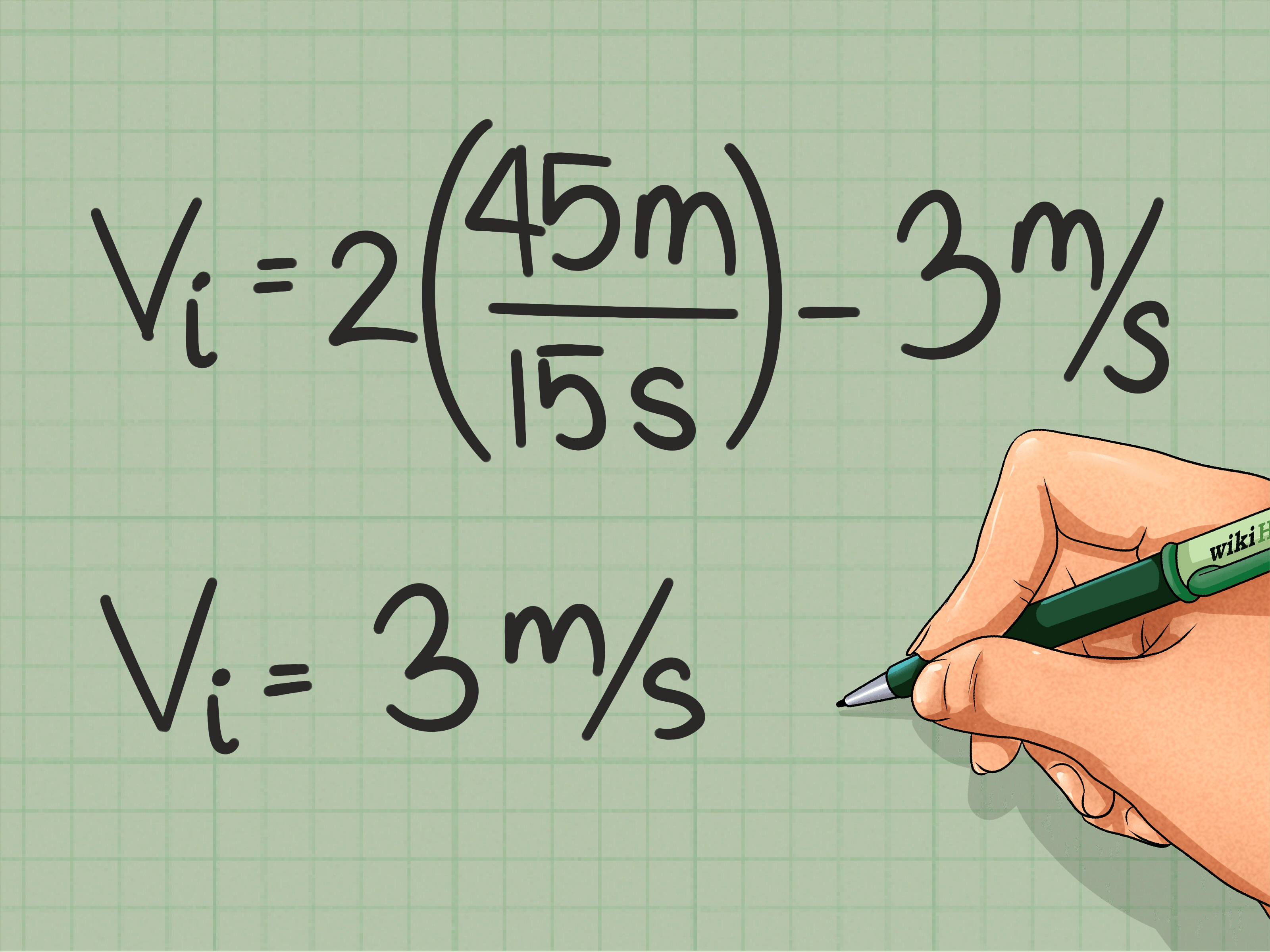
vi = 2(Δx/t) − vf
Example: A cart on a straight track
A cart travels 84 meters in 6 seconds and finishes at 18 m/s. Assuming constant acceleration, find its initial velocity.
- Calculate average velocity: vavg = 84/6 = 14 m/s.
- Use vi = 2vavg − vf.
- Substitute: vi = 2(14) − 18 = 10 m/s.
Answer: The cart’s initial velocity was 10 m/s.
Because the cart accelerates uniformly from 10 m/s to 18 m/s, its average velocity is halfway between them: 14 m/s. Multiplying 14 m/s by 6 seconds reproduces the 84-meter displacement.
Be careful: the simple average of initial and final velocity is valid for constant acceleration. It is not automatically valid when an object accelerates irregularly.
How to Choose Among the Four Initial Velocity Formulas
| Known information | Formula for initial velocity | Variable omitted |
|---|---|---|
| Final velocity, acceleration, time | vi = vf − at | Displacement |
| Displacement, acceleration, time | vi = Δx/t − ½at | Final velocity |
| Final velocity, acceleration, displacement | vi = ±√(vf2 − 2aΔx) | Time |
| Final velocity, displacement, time | vi = 2Δx/t − vf | Acceleration |
The easiest selection rule is to circle the known quantities. Find the row containing those three values, and use its equation. This approach is more dependable than memorizing equations by number because textbooks do not always number them in the same order.
Finding Initial Velocity in Projectile Motion
Projectile motion is two-dimensional, but the same kinematic formulas still work after the motion is separated into horizontal and vertical components. If a projectile is launched at speed v0 and angle θ above the horizontal, its starting components are:
v0x = v0 cos θ
v0y = v0 sin θ
Ignoring air resistance, horizontal acceleration is zero, while vertical acceleration near Earth’s surface is approximately −9.8 m/s2 when upward is positive.
Suppose the initial components have been calculated as 12 m/s horizontally and 9 m/s vertically. The magnitude of the launch velocity is:
v0 = √(122 + 92) = 15 m/s
The direction is:
θ = tan−1(9/12) ≈ 36.9°
Always solve the horizontal and vertical motions separately before recombining them. Stuffing both directions into one one-dimensional equation is a reliable way to invent a new branch of physics that no professor requested.
Common Mistakes When Calculating Initial Velocity
Ignoring direction
A negative velocity is not inherently wrong. It simply points opposite the chosen positive direction. Write down your coordinate convention before calculating.
Using distance instead of displacement
Kinematic equations use displacement. Distance and displacement are identical only when an object travels in one direction without reversing.
Mixing units
Seconds, meters, and meters per second belong together. Convert minutes to seconds, kilometers to meters, or mph to m/s before substitution.
Forgetting the square on time
In Δx = vit + ½at2, only the time in the acceleration term is squared. Losing that exponent changes both the units and the answer.
Assuming constant acceleration without checking
The four formulas describe uniform acceleration. They are not exact for a car whose driver alternates between the gas and brake pedals, an object experiencing strong air resistance, or any motion with substantially changing acceleration.
Rounding too early
Keep extra digits during intermediate steps and round the final result. Otherwise, several innocent-looking approximations can team up and mug your answer.
Practical Experiences and Lessons from Initial Velocity Problems
Working through initial velocity problems reveals that algebra is rarely the hardest part. The real challenge is translating a physical story into a consistent mathematical model. A student may know every kinematic equation on the formula sheet and still struggle if “slowing westward” has not been converted into signed quantities.
One particularly useful experience is analyzing a rolling ball with a phone camera. Place distance markers beside a straight path, record the ball, and note its position at several timestamps. A position-versus-time graph can then be fitted with a quadratic model of the form x(t) = x0 + vit + ½at2. The coefficient of t represents initial velocity, while twice the coefficient of t2 represents acceleration. Suddenly, the formula is no longer decorative classroom wallpaper; it describes visible motion.
This experiment also exposes the difference between ideal equations and imperfect measurements. Video may record at an uncertain frame rate, markers may not be evenly spaced, and the ball may encounter small bumps or friction changes. Calculated velocities can vary slightly depending on which observations are used. That variation is not necessarily failure. It is evidence that models simplify reality and measurements contain uncertainty.
A second valuable experience comes from checking one solution with another equation. After using final velocity, acceleration, and time to calculate vi, use the result to predict displacement. If the predicted displacement matches the information in the problem, confidence in the answer rises. If it does not, inspect the signs, units, and arithmetic. Physics problems are much easier when equations act as one another’s proofreaders.
Vertical-motion exercises provide a memorable lesson about signs. Toss a ball upward while defining upward as positive. Its initial velocity is positive, but gravitational acceleration is negative. At the highest point, the vertical velocity is zero, yet acceleration remains −9.8 m/s2. Many beginners assume everything becomes zero at the top. Watching a slow-motion recording helps correct that idea: the ball pauses only instantaneously before gravity continues changing its velocity downward.
Another practical lesson is to estimate before calculating. If a car reaches 30 m/s after gaining roughly 10 m/s, its starting velocity should be near 20 m/s. An answer of 200 m/s is then an obvious warning, even if every calculator button was pressed with magnificent confidence. Estimation catches misplaced decimals, forgotten negative signs, and unit conversions that wandered off course.
Repeated practice also makes formula selection feel less like memorization. Instead of asking, “Which of the four equations was number three?” ask, “What do I know, what do I need, and which variable should be absent?” If time is not given, choose the equation without time. If acceleration is unknown, use displacement, time, and average velocity. This variable-based habit transfers naturally to more advanced physics.
Finally, real experiments teach humility about significant figures. A time measured as 4.2 seconds does not justify reporting initial velocity as 13.428571 m/s. The additional digits imply precision the experiment never had. A result such as 13 m/s, or perhaps 13.4 m/s when the data support it, is more honest and easier to interpret.
The broader experience is that finding initial velocity is not just equation rearrangement. It involves defining a reference direction, recognizing assumptions, interpreting data, checking physical plausibility, and communicating a result with appropriate units. Master those habits, and the formulas become useful tools instead of cryptic arrangements of letters.
Conclusion
There are four straightforward ways to find initial velocity under constant acceleration. The correct method depends on whether the known information includes time, displacement, acceleration, or final velocity. List the variables, establish a positive direction, select the equation that excludes the missing quantity, and check the result against the physical situation.
Initial velocity calculations become far more manageable once signs and units are treated as part of the physics rather than paperwork added at the end. A sensible answer should have velocity units, follow the chosen direction convention, and reproduce the known motion when substituted back into the original equation.